This vignette documents a sample analysis of Triple Negative Breast Cancer (TNBC) data, retrieved from . We consider the classified phenotypes rather than the direct protein data, pre-loaded in this package.
TNBC_pheno <- TNBC_pheno
TNBC_meta <- TNBC_meta
We begin by defining the phenotypes of interest as well as the related interactions.
phenos <- unique(TNBC_pheno$Phenotype)
pheno_interactions <- rbind(
  data.frame(t(combn(phenos, 2))),
  data.frame("X1" = phenos, "X2" = phenos)
)

phenos_subset <- c(
  "Tumor", "CD3T", "CD4T", "CD8T", "B", "DC",
  "DCMono", "Macrophage", "MonoNeu", "NK", "Treg"
)
pheno_interactions_subset <- data.frame(
  Var1 = rep("Tumor", 11),
  Var2 = c(
    "Tumor", "CD3T", "CD4T", "CD8T", "B", "DC",
    "DCMono", "Macrophage", "MonoNeu", "NK", "Treg"
  )
)
We notice there are 16 total phenotypes with 136 total possible interactions. Alternatively, we can also focus on a subset of phenotypes (11) and interactions (11) of particular interest. Another analysis on the subset interaction set has been considered but was suppressed for brevity.
In order to build confidence in our approach, we begin by simulating data with a similar structure to the full phenotype data and evaluating the effectiveness of the approach.
To start, let us determine the agent information in a typical image.
data_pheno_stat <- data.frame("pheno" = phenos)
for (person in unique(TNBC_pheno$Person)) {
  tmp <- as.data.frame(table(TNBC_pheno[TNBC_pheno$Person == person, "Phenotype"]))
  colnames(tmp) <- c("pheno", person)
  data_pheno_stat <- merge(x = data_pheno_stat, y = tmp, all.x = TRUE)
}

agent_info_subset <- data.frame(data_pheno_stat[1],
  "mean" = rowMeans(data_pheno_stat[-1], na.rm = TRUE),
  "med" = apply(data_pheno_stat[-1], 1, median, na.rm = TRUE)
)
Now let us generate two data sets: (1) where no informative interactions are present and (2) where some informative interactions are present. We generate \(34\) patients, comparative to the 33 TNBC patients. We generate \(15\) for each class with possible interactions, if present, and \(2\) for each class that are indistinguishable to add some noise to the data.
The non-interactive data is simulated as follows.
set.seed(123)
dat0 <- simulatePP(
  agentVarData =
    data.frame(
      "outcome" = c(0, 1),
      "c1" = c(0, 0),
      "c2" = c(1 / 25, 1 / 25), "c3" = c(1 / 50, 1 / 50),
      "c4" = c(0, 0),
      "c5" = c(0, 0), "c6" = c(0, 0),
      "c7" = c(0, 0), "c8" = c(1 / 100, 1 / 100),
      "c9" = c(1 / 20, 1 / 20), "c10" = c(1 / 250, 1 / 250),
      "c11" = c(1 / 100, 1 / 100), "c12" = c(1 / 80, 1 / 80),
      "c13" = c(0, 0), "c14" = c(0, 0),
      "c15" = c(0, 0), "c16" = c(1 / 10, 1 / 10)
    ),
  agentKappaData = data.frame(
    "agent" = paste0("c", 1:16),
    "clusterAgent" = c(NA, "c1", "c1", rep(NA, 12), "c1"),
    "kappa" = c(
      rbinom(1, 100, 0.5),
      rbinom(1, 100, 0.5),
      rbinom(1, 30, 0.5),
      rbinom(1, 80, 0.5),
      rbinom(1, 350, 0.5),
      rbinom(1, 100, 0.5),
      rbinom(1, 120, 0.5),
      rbinom(1, 150, 0.5),
      rbinom(2, 250, 0.5),
      rbinom(1, 600, 0.5),
      rbinom(1, 60, 0.5),
      rbinom(2, 140, 0.5),
      rbinom(1, 20, 0.5),
      rbinom(1, 5, 0.5)
    )
  ),
  unitsPerOutcome = 15,
  replicatesPerUnit = 1,
  silent = FALSE
)
#> Outcome: 0 (1/2)
#> Outcome: 1 (2/2)
dat1 <- simulatePP(
  agentVarData =
    data.frame(
      "outcome" = c(0, 1),
      "c1" = c(0, 0),
      "c2" = c(1 / 25, 1 / 25), "c3" = c(1 / 50, 1 / 50),
      "c4" = c(0, 0),
      "c5" = c(0, 0), "c6" = c(0, 0),
      "c7" = c(0, 0), "c8" = c(1 / 100, 1 / 100),
      "c9" = c(1 / 20, 1 / 20), "c10" = c(1 / 250, 1 / 250),
      "c11" = c(1 / 100, 1 / 100), "c12" = c(1 / 80, 1 / 80),
      "c13" = c(0, 0), "c14" = c(0, 0),
      "c15" = c(0, 0), "c16" = c(1 / 10, 1 / 10)
    ),
  agentKappaData = data.frame(
    "agent" = paste0("c", 1:16),
    "clusterAgent" = c(NA, "c1", "c1", rep(NA, 12), "c1"),
    "kappa" = c(
      rbinom(1, 100, 0.5),
      rbinom(1, 100, 0.5),
      rbinom(1, 30, 0.5),
      rbinom(1, 80, 0.5),
      rbinom(1, 350, 0.5),
      rbinom(1, 100, 0.5),
      rbinom(1, 120, 0.5),
      rbinom(1, 150, 0.5),
      rbinom(2, 250, 0.5),
      rbinom(1, 600, 0.5),
      rbinom(1, 60, 0.5),
      rbinom(2, 140, 0.5),
      rbinom(1, 20, 0.5),
      rbinom(1, 5, 0.5)
    )
  ),
  unitsPerOutcome = 2,
  replicatesPerUnit = 1,
  silent = F
)
#> Outcome: 0 (1/2)
#> Outcome: 1 (2/2)
dat1$unit <- ifelse(dat1$unit == "u1", "u31",
  ifelse(dat1$unit == "u2", "u32",
    ifelse(dat1$unit == "u3", "u33",
      ifelse(dat1$unit == "u4", "u34", NA)
    )
  )
)
dat1$replicate <- ifelse(dat1$replicate == "1", "31",
  ifelse(dat1$replicate == "2", "32",
    ifelse(dat1$replicate == "3", "33",
      ifelse(dat1$replicate == "4", "34", NA)
    )
  )
)
dat <- rbind(dat0, dat1)
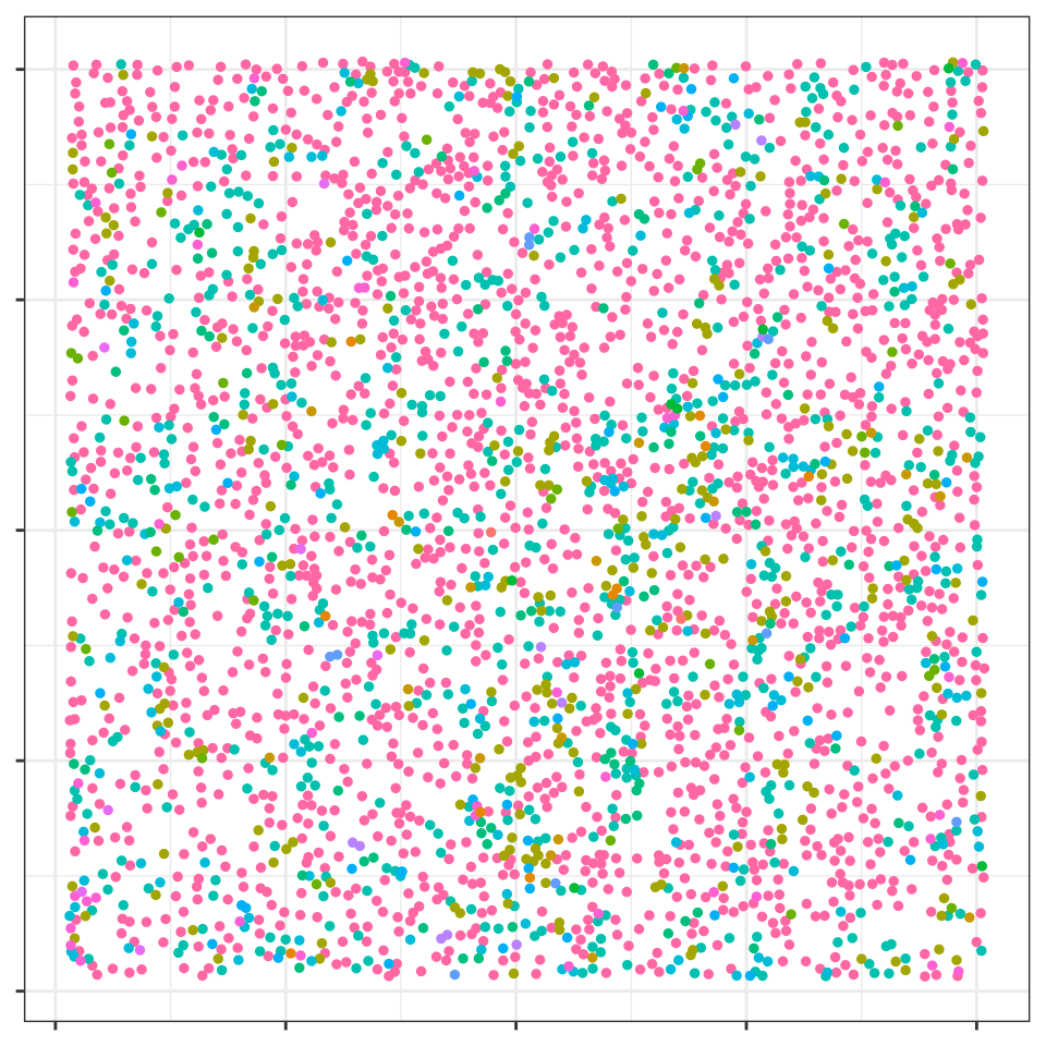
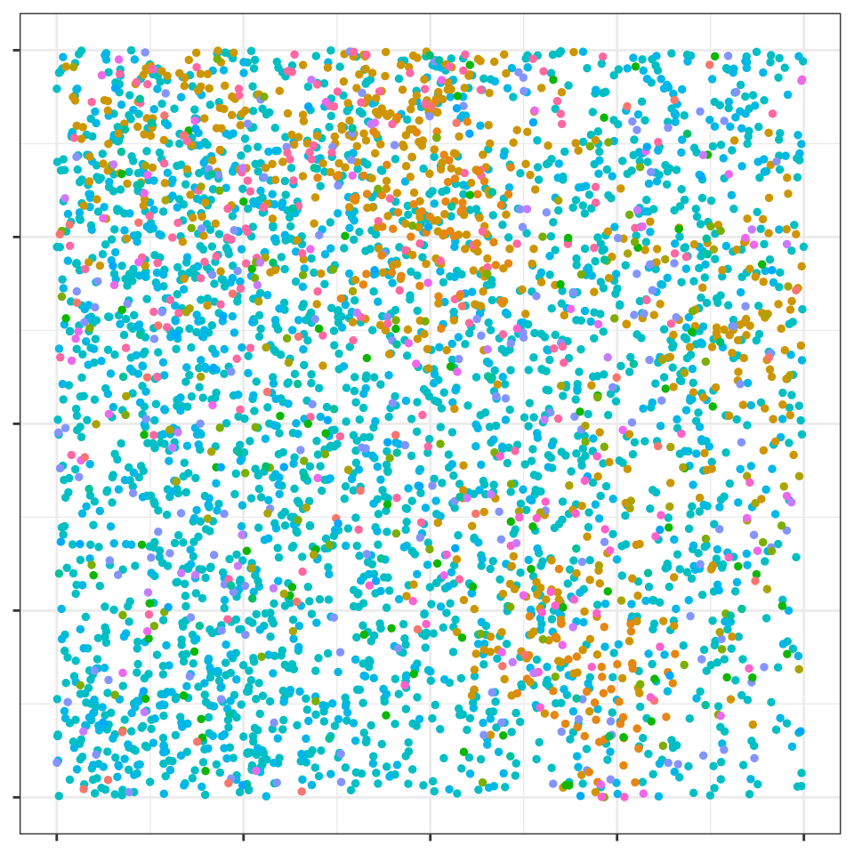
Compare images of the data.
plotPP(
  data = TNBC_pheno[TNBC_pheno$Person == 2, c("cellx", "celly", "Phenotype")],
  ptSize = 1, dropAxes = T, colorGuide = "none"
)
TNBC Patient Image
plotPP(dat[dat$replicate == 18, c("x", "y", "type")],
  ptSize = 1, dropAxes = T, colorGuide = "none"
)
Simulated Patient Image
Now we compute PCA and attach an age meta-variable (with no effect).
cells <- paste0("c", 1:16)
cells_interactions <- rbind(
  data.frame(t(combn(cells, 2))),
  data.frame("X1" = cells, "X2" = cells)
)

set.seed(12345)
pcaData <- getKsPCAData(
  data = dat, replicate = "replicate",
  agents_df = cells_interactions,
  xRange = c(0, 1), yRange = c(0, 1),
  silent = F
)
pcaMeta <- simulateMeta(pcaData,
  metaInfo = data.frame(
    "var" = c("age"),
    "rdist" = c("rnorm"),
    "outcome_0" = c("25"),
    "outcome_1" = c("25")
  )
)
We analyze the data.
set.seed(123)
rfcv <- funkyModel(
  data = pcaMeta,
  outcome = "outcome",
  unit = "unit",
  metaNames = c("age")
)
Resulting in the variable importance figures. The code for these is given below, but may not be shown due to computational time in creating this vignette.
rfcv$viPlot
rfcv$subset_viPlotNow we consider the simulated model with effects.
set.seed(123456)
dat0 <- simulatePP(
  agentVarData =
    data.frame(
      "outcome" = c(0, 1),
      "c1" = c(0, 0),
      "c2" = c(1 / 25, 1 / 60), "c3" = c(1 / 50, 1 / 10),
      "c4" = c(0, 0),
      "c5" = c(0, 0), "c6" = c(0, 0),
      "c7" = c(0, 0), "c8" = c(1 / 100, 1 / 100),
      "c9" = c(1 / 20, 1 / 20), "c10" = c(1 / 250, 1 / 250),
      "c11" = c(1 / 100, 1 / 100), "c12" = c(1 / 80, 1 / 80),
      "c13" = c(0, 0), "c14" = c(0, 0),
      "c15" = c(0, 0), "c16" = c(1 / 10, 1 / 10)
    ),
  agentKappaData = data.frame(
    "agent" = paste0("c", 1:16),
    "clusterAgent" = c(NA, "c1", "c1", rep(NA, 12), "c1"),
    "kappa" = c(
      rbinom(1, 100, 0.5),
      rbinom(1, 100, 0.5),
      rbinom(1, 30, 0.5),
      rbinom(1, 80, 0.5),
      rbinom(1, 350, 0.5),
      rbinom(1, 100, 0.5),
      rbinom(1, 120, 0.5),
      rbinom(1, 150, 0.5),
      rbinom(2, 250, 0.5),
      rbinom(1, 600, 0.5),
      rbinom(1, 60, 0.5),
      rbinom(2, 140, 0.5),
      rbinom(1, 20, 0.5),
      rbinom(1, 5, 0.5)
    )
  ),
  unitsPerOutcome = 15,
  replicatesPerUnit = 1,
  silent = F
)
dat1 <- simulatePP(
  agentVarData =
    data.frame(
      "outcome" = c(0, 1),
      "c1" = c(0, 0),
      "c2" = c(1 / 25, 1 / 25), "c3" = c(1 / 50, 1 / 50),
      "c4" = c(0, 0),
      "c5" = c(0, 0), "c6" = c(0, 0),
      "c7" = c(0, 0), "c8" = c(1 / 100, 1 / 100),
      "c9" = c(1 / 20, 1 / 20), "c10" = c(1 / 250, 1 / 250),
      "c11" = c(1 / 100, 1 / 100), "c12" = c(1 / 80, 1 / 80),
      "c13" = c(0, 0), "c14" = c(0, 0),
      "c15" = c(0, 0), "c16" = c(1 / 10, 1 / 10)
    ),
  agentKappaData = data.frame(
    "agent" = paste0("c", 1:16),
    "clusterAgent" = c(NA, "c1", "c1", rep(NA, 12), "c1"),
    "kappa" = c(
      rbinom(1, 100, 0.5),
      rbinom(1, 100, 0.5),
      rbinom(1, 30, 0.5),
      rbinom(1, 80, 0.5),
      rbinom(1, 350, 0.5),
      rbinom(1, 100, 0.5),
      rbinom(1, 120, 0.5),
      rbinom(1, 150, 0.5),
      rbinom(2, 250, 0.5),
      rbinom(1, 600, 0.5),
      rbinom(1, 60, 0.5),
      rbinom(2, 140, 0.5),
      rbinom(1, 20, 0.5),
      rbinom(1, 5, 0.5)
    )
  ),
  unitsPerOutcome = 2,
  replicatesPerUnit = 1,
  silent = F
)
dat1$unit <- ifelse(dat1$unit == "u1", "u31",
  ifelse(dat1$unit == "u2", "u32",
    ifelse(dat1$unit == "u3", "u33",
      ifelse(dat1$unit == "u4", "u34", NA)
    )
  )
)
dat1$replicate <- ifelse(dat1$replicate == "1", "31",
  ifelse(dat1$replicate == "2", "32",
    ifelse(dat1$replicate == "3", "33",
      ifelse(dat1$replicate == "4", "34", NA)
    )
  )
)
dat <- rbind(dat0, dat1)

cells <- paste0("c", 1:16)
cells_interactions <- rbind(
  data.frame(t(combn(cells, 2))),
  data.frame("X1" = cells, "X2" = cells)
)

pcaData <- getKsPCAData(
  data = dat, replicate = "replicate",
  agents_df = cells_interactions,
  xRange = c(0, 1), yRange = c(0, 1),
  silent = F
)
pcaMeta <- simulateMeta(pcaData,
  metaInfo = data.frame(
    "var" = c("age"),
    "rdist" = c("rnorm"),
    "outcome_0" = c("25"),
    "outcome_1" = c("27")
  )
)

rfcv <- funkyModel(
  data = pcaMeta,
  outcome = "outcome",
  unit = "unit",
  metaNames = c("age")
)
Creating the variable importance plots as before (code below, perhaps figure not given for computational reasons)
rfcv$viPlot
rfcv$subset_viPlotWith this confidence, we now consider the TNBC phenotype data.
dataPCA_pheno <- getKsPCAData(
  data = TNBC_pheno, unit = "Person",
  agents_df = pheno_interactions,
  rCheckVals = seq(0, 50, 1)
)

dataPCAAge_pheno <- merge(dataPCA_pheno, TNBC_meta)

set.seed(123456)
rfcv <- funkyModel(
  data = dataPCAAge_pheno, K = 10,
  outcome = "Class", unit = "Person",
  metaNames = c("Age"), synthetics = 100,
  alpha = 0.05, silent = FALSE,
  subsetPlotSize = 25
)
And the related variable importance plots (may not be shown for computational reasons).
rfcv$viPlot
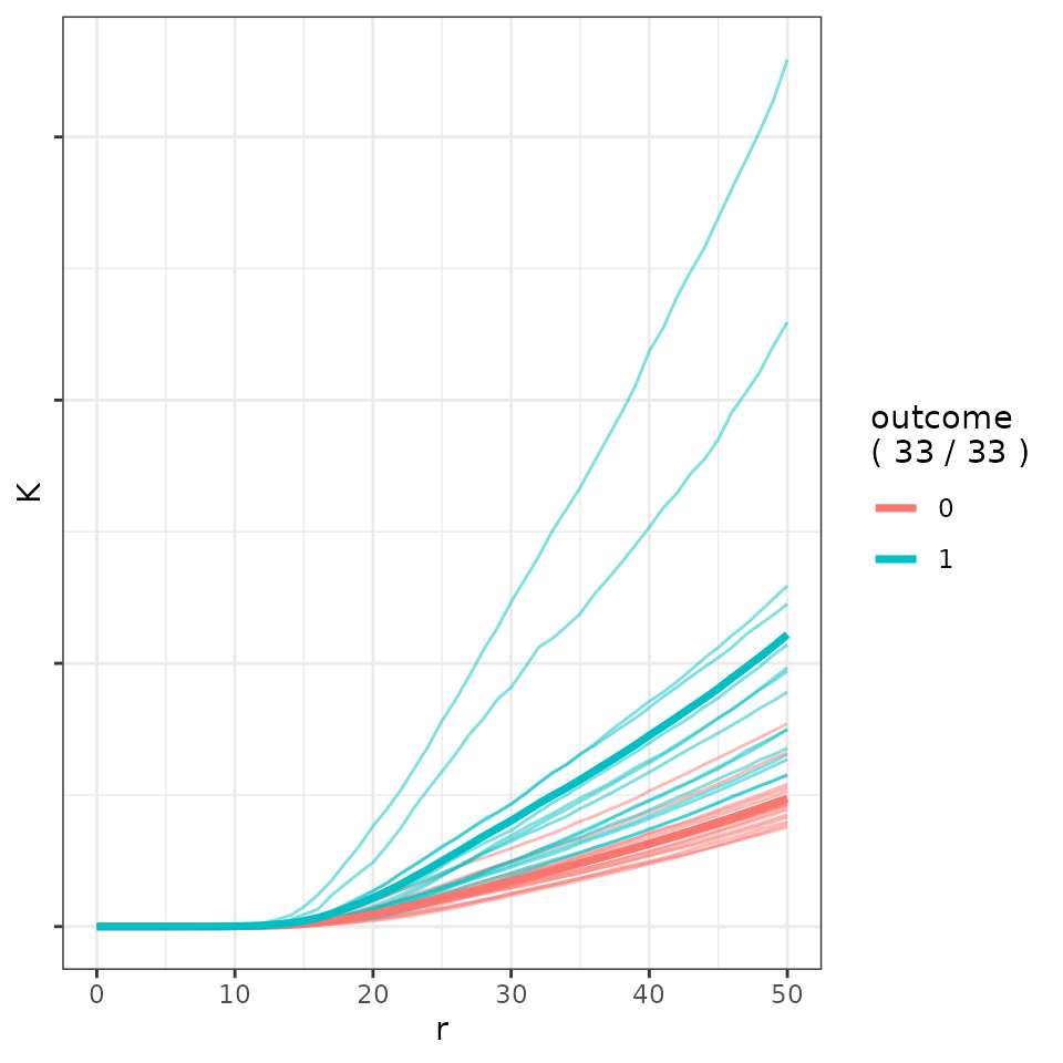
rfcv$subset_viPlotAlso consider \(K\) functions from significant and insignificant interactions.
tmp <- getKFunction(TNBC_pheno[TNBC_pheno$Class == 0, -1],
  c("Tumor", "Tumor"),
  unit = "Person",
  rCheckVals = seq(0, 50, 1)
)
tmp1 <- getKFunction(TNBC_pheno[TNBC_pheno$Class == 1, -1],
  c("Tumor", "Tumor"),
  unit = "Person",
  rCheckVals = seq(0, 50, 1)
)

tmp_1 <- tidyr::pivot_longer(data = tmp, cols = -r)
tmp1_1 <- tidyr::pivot_longer(data = tmp1, cols = -r)

data_plot <- rbind(
  data.frame(
    "r" = tmp_1$r,
    "K" = tmp_1$value,
    "unit" = tmp_1$name,
    "outcome" = "0"
  ),
  data.frame(
    "r" = tmp1_1$r,
    "K" = tmp1_1$value,
    "unit" = paste0(tmp1_1$name, "_1"),
    "outcome" = "1"
  )
)
Creating the following figure.
plot_K_functions(data_plot)
TNBC Phenotype Significant K Function
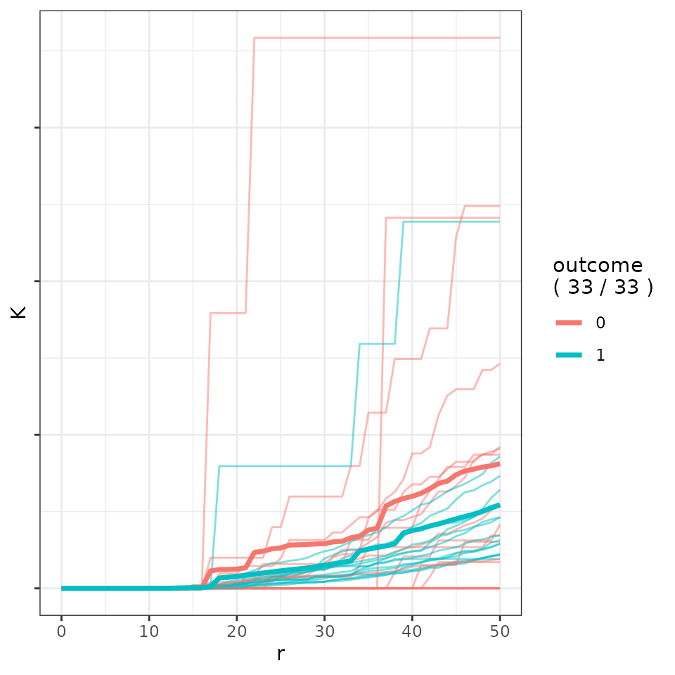
And for a insignificant interaction.
tmp <- getKFunction(TNBC_pheno[TNBC_pheno$Class == 0, -1],
  c("CD4T", "Endothelial"),
  unit = "Person",
  rCheckVals = seq(0, 50, 1)
)
tmp1 <- getKFunction(TNBC_pheno[TNBC_pheno$Class == 1, -1],
  c("CD4T", "Endothelial"),
  unit = "Person",
  rCheckVals = seq(0, 50, 1)
)

tmp_1 <- tidyr::pivot_longer(data = tmp, cols = -r)
tmp1_1 <- tidyr::pivot_longer(data = tmp1, cols = -r)

data_plot <- rbind(
  data.frame(
    "r" = tmp_1$r,
    "K" = tmp_1$value,
    "unit" = tmp_1$name,
    "outcome" = "0"
  ),
  data.frame(
    "r" = tmp1_1$r,
    "K" = tmp1_1$value,
    "unit" = paste0(tmp1_1$name, "_1"),
    "outcome" = "1"
  )
)
Creating the following figure.
plot_K_functions(data_plot)
TNBC Phenotype Insignficant K Function
Further analysis of this data can be found in our paper.