cats

Overview

This article examines data on cats, includes as cats and subcats in the package. The goal of this analysis is to see the effect sex has on the body and heart weight measures. This analysis goes further than that in the purify article by adding cross-validation to the summary function. This comes at the cost of computational time.

library(purify)
library(ggplot2)

summ_function <- function(data) {
  cv <- cross_validation(
    data = data,
    pred_fn = function(data, nd) {
      as.numeric(predict(lm(Hwt ~ ., data = data), newdata = nd))
    },
    error_fn = function(true, est) {
      mean((true$Hwt - est)^2)
    }
  )
  mod <- lm(Hwt ~ ., data = data)
  c(cv[[1]], as.numeric(coef(summary(mod))[, 1]))
}

Full Data

We first are interested in the coefficients when estimating the body weight using sex and heart weight, stratified on sex since there are far less female cats observed.

plot_strata_bar(cats$Sex)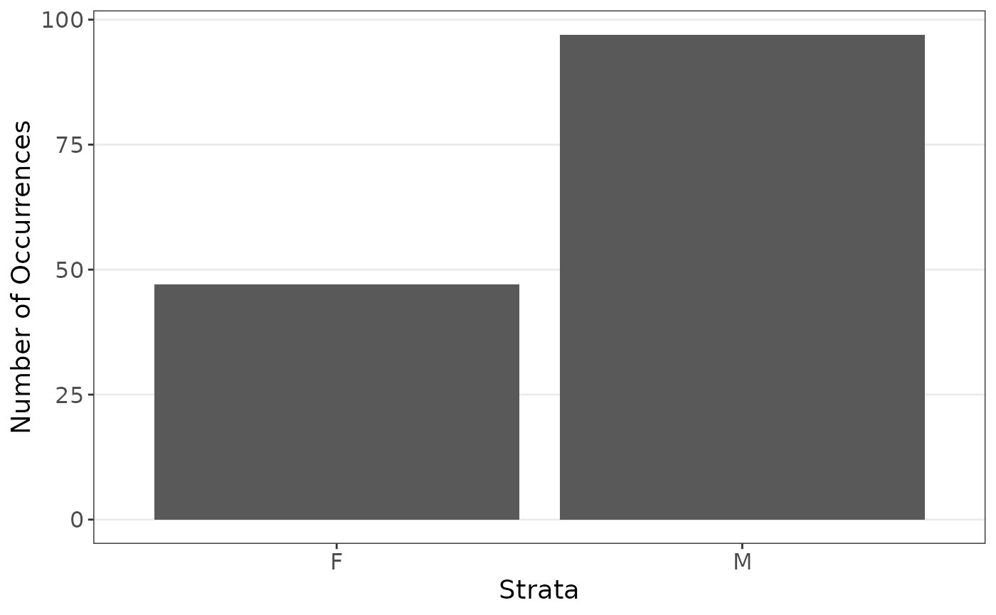

plot_strata_box(cats[, c("Sex", "Hwt")])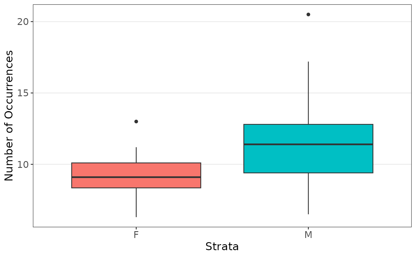

plot_strata_box(cats[, c("Sex", "Bwt")])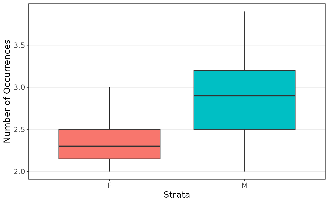

ggplot() +
  geom_point(aes(x = Bwt, y = Hwt, col = Sex, shape = Sex), data = cats, size = 5) +
  theme_bw() +
  theme(
    axis.title = element_text(size = 30),
    axis.text = element_text(size = 26),
    legend.position = c(.2, .8),
    legend.title = element_blank(),
    legend.text = element_text(size = 26)
  ) +
  scale_color_discrete(labels = c("Female", "Male")) +
  scale_shape_manual(
    labels = c("Female", "Male"),
    values = c(16, 3)
  ) +
  xlab("Body weight (kg)") +
  ylab("Heart weight (g)")
#> Warning: A numeric `legend.position` argument in `theme()` was deprecated in ggplot2
#> 3.5.0.
#> ℹ Please use the `legend.position.inside` argument of `theme()` instead.
#> This warning is displayed once every 8 hours.
#> Call `lifecycle::last_lifecycle_warnings()` to see where this warning was
#> generated.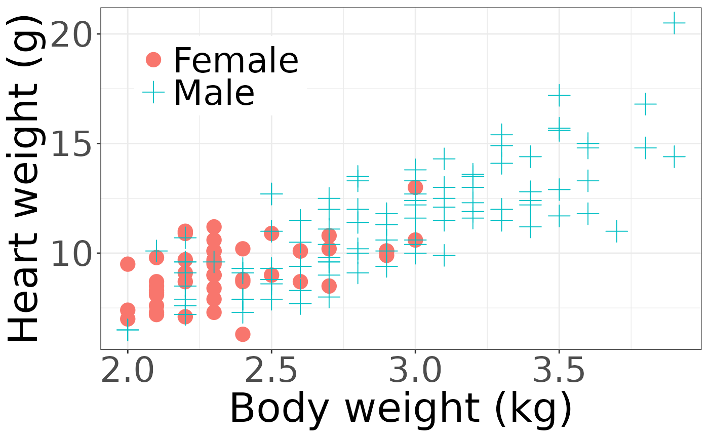

Now modeling the data:

set.seed(1234)
summ_function(cats)
#> [1]  2.18141845 -0.41495263 -0.08209684  4.07576892

# Perform resampling (with CV included so a bit time consuming)
results <- resample(
  data = cats, fn = summ_function, M = 500,
  strata = "Sex", sizes = mean
)
summarize_resample(results)
#>     estimates        sd      lower     upper
#> V1 1.94170124 0.2396958  1.5219943 2.4252585
#> V2 0.09127577 0.9101625 -1.7096981 1.6920913
#> V3 0.04491171 0.2672944 -0.4863061 0.5720345
#> V4 3.86256391 0.3790560  3.2023760 4.6366714

In both methods, the sex was insignificant and body weight was important.

Subset Data

We are now interested in the coefficients when estimating the body weight using sex and heart weight, stratified on sex since there are far less female cats observed, with a smaller data set. In practice it is hard to know the exact effect of data sizes, so it is worth examining what may happen. We subset the data such that sex will now be more important

plot_strata_bar(subcats$Sex)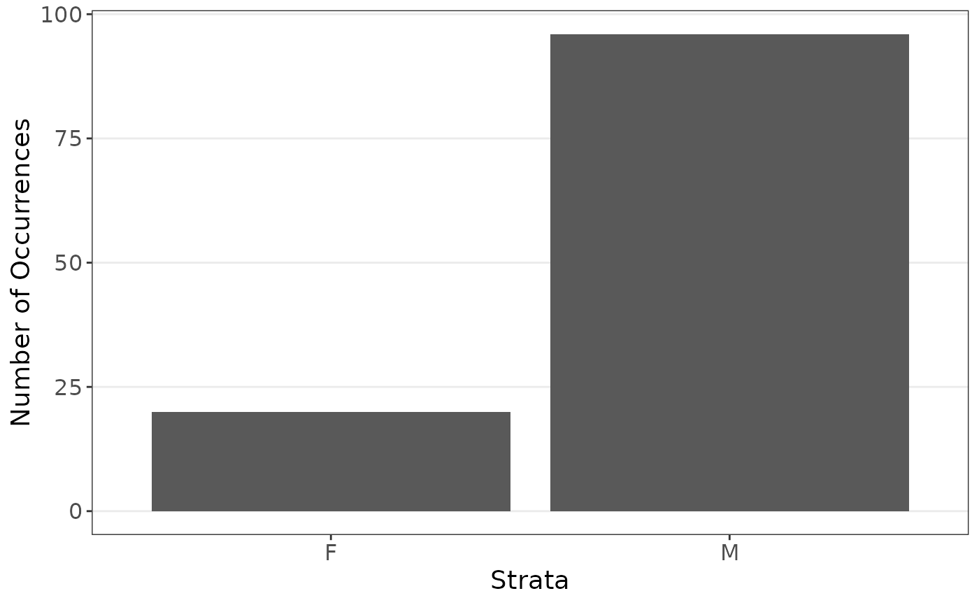

Now modeling the data:

# Original model
set.seed(1234)
tmp <- lm(Hwt ~ ., data = subcats)
coef(summary(tmp))
#>               Estimate Std. Error   t value     Pr(>|t|)
#> (Intercept) -1.4861533  0.8831869 -1.682717 9.519112e-02
#> SexM         0.6167464  0.3812708  1.617607 1.085354e-01
#> Bwt          4.2078878  0.3204588 13.130823 1.760509e-24
confint(tmp)
#>                  2.5 %    97.5 %
#> (Intercept) -3.2359058 0.2635992
#> SexM        -0.1386197 1.3721126
#> Bwt          3.5730011 4.8427744

## CV for both
set.seed(1234)
results <- resample(
  data = subcats, fn = summ_function,
  M = 500, strata = "Sex"
)

cross_validation(
  data = subcats,
  pred_fn = function(data, nd) {
    as.numeric(predict(lm(Hwt ~ ., data = data), newdata = nd))
  },
  error_fn = function(true, est) {
    mean((true$Hwt - est)^2)
  }
)
#>      est       sd 
#> 2.257610 3.497294
summarize_resample(results)
#>     estimates        sd       lower     upper
#> V1  2.1993929 0.3018411  1.66413178 2.7710629
#> V2 -1.4264232 1.0870510 -3.64402987 0.6916344
#> V3  0.6192422 0.2750080  0.04371714 1.1632974
#> V4  4.1885264 0.4146341  3.41731140 5.0068961

In examining the data, we can observe that sex is important, but is hard to see due to the low samples. Traditional linear models miss this; however, a resampled method can capture the importance of sex without losing the effects of body weight. The resampled method also improves estimation in terms of mean squared error.