Functional Spherical Autocorrelation Function

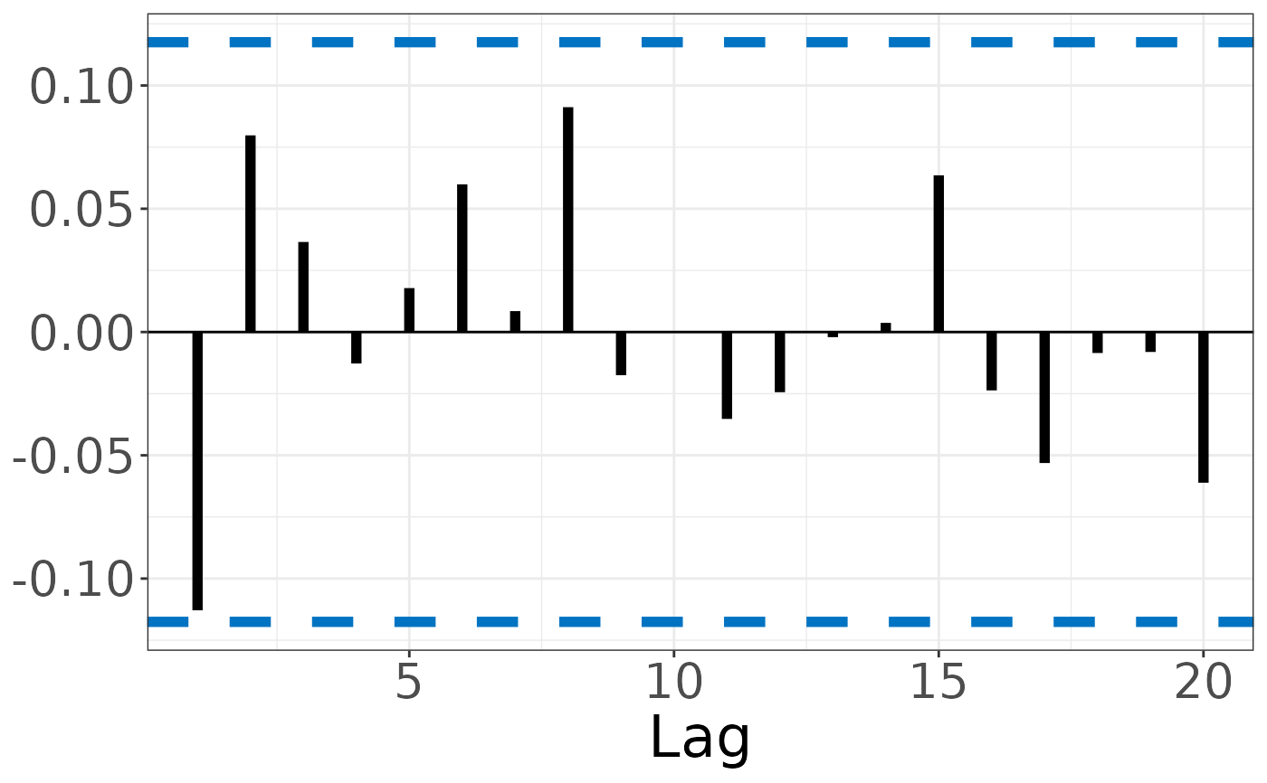
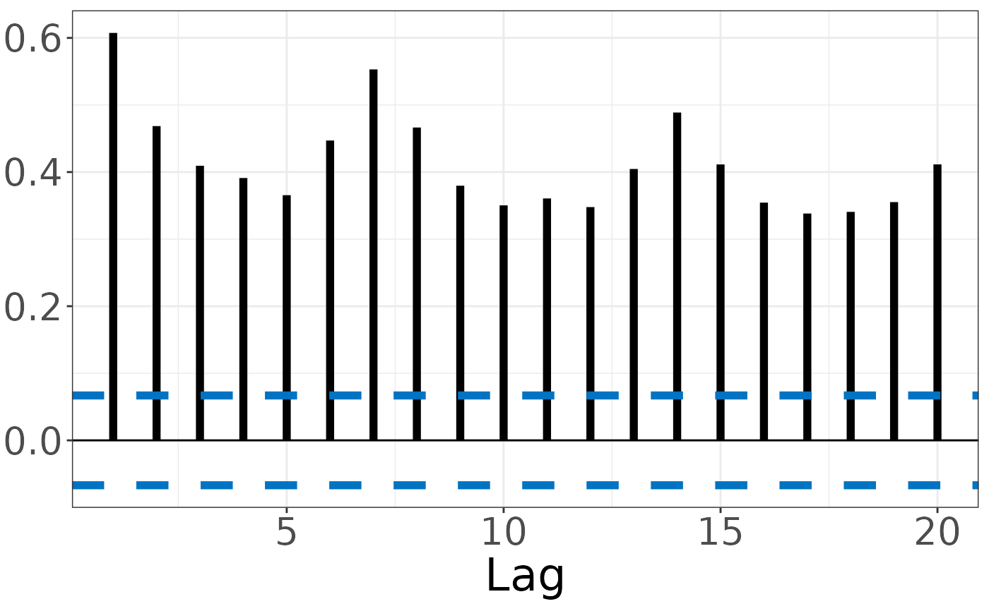
This function offers a graphical summary of the fSACF of a functional time series (FTS) across different time lags \(h = 1:H\). It also plots \(100 \times (1-\alpha)\%\) confidence bounds developed under strong white noise (SWN) assumption for all lags \(h = 1:H\).

Usage

sacf(X, lag.max = 20, alpha = 0.05, figure = TRUE)

Arguments

X

A dfts object or data which can be automatically converted to that format. See dfts().

lag.max

A positive integer value. The maximum lag for which to compute the coefficients and confidence bounds.

alpha

Significance in [0,1] for intervals when forecasting.

figure

Logical. If TRUE, prints plot for the estimated function with the specified bounds.

Value

List with sACF values and plots

Details

This function computes and plots functional spherical autocorrelation coefficients at lag \(h\), for \(h = 1:H\). The fSACF at lag \(h\) is computed by the average of the inner product of lagged pairs of the series \(X_i\) and \(X_{i+h}\) that have been centered and scaled: $$ \tilde\rho_h=\frac{1}{N}\sum_{i=1}^{N-h} \langle \frac{X_i - \tilde{\mu}}{\|X_i - \tilde{\mu}\|}, \frac{X_{i+h} - \tilde{\mu}}{\|X_{i+h} - \tilde{\mu}\|} \rangle,\ \ \ \ 0 \le h < N, $$ where \(\tilde{\mu}\) is the estimated spatial median of the series. It also computes estimated asymptotic \((1-\alpha)100 \%\) confidence lower and upper bounds, under the SWN assumption.

References

Yeh C.K., Rice G., Dubin J.A. (2023). Functional spherical autocorrelation: A robust estimate of the autocorrelation of a functional time series. Electronic Journal of Statistics, 17, 650–687.

See also

acf()

Examples

sacf(electricity)

sacf(generate_brownian_motion(100) )